Nvidia Stock Analysis
This project involves analyzing financial data to uncover trends and insights.
Key takeaways from the analysis
- The recent dip below both SMAs and MACD bearish crossover hint at a possible trend reversal.
- Nvidia has displayed strong historical outperformance, but volatily remains high.
- Market sentiment has shifted due to AI sector competition and earnings call uncertainty.
- Risk-adjusted returns remain favorable (Sharpe Ratio: 1.83), but investors should be cautious given high drawdowns and expected price volatility.
- Monte Carlo simulations predict significant price fluctuations, reinforcing the need for active risk management.
- The recent earnings announcement has had a significant impact on stock price and trading patterns, underscoring the importance of fundamental analysis alongside technical indicators.
Trend Analysis with Moving Averages
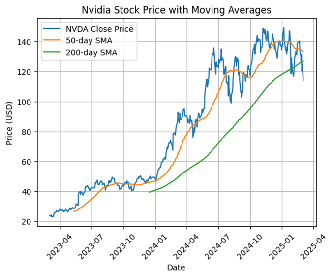
Over the past two years, Nvidia stock followed a strong uptrend. However, in recent days, the stock price has fallen below both the 50-day and 200-day Simple Moving Averages (SMA). The proximity of these SMAs also suggest a possible bearish crossover, potentially signaling a trend reversal.
If the 50-day SMA crosses below the 200-day SMA, further downside pressure may emerge. However, investors should also watch for any false signals and confirm the trend with additional indicators. The stocks’ reaction to the late February earnings call has been particularly notable, with significant price movements observed in the days following the announcement.
Momentum and Overbought/Oversold Conditions
MACD Analysis
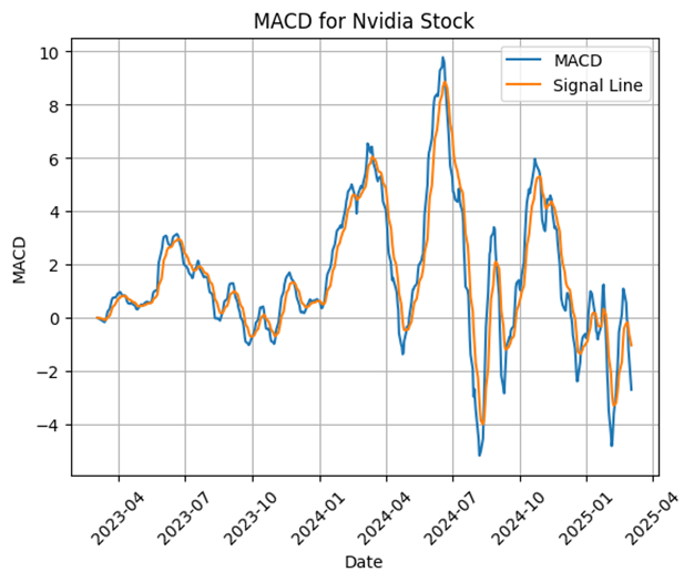
The Moving Average Convergence Divergence (MACD) indicator shows that Nvidia's momentum has recently weakened. The MACD line appears bellow the signal line, which indicates a bearish trend continuation. This might support the bearish crossover observe in the SMAs.
RSI Analysis
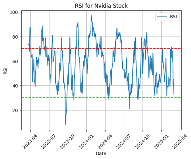
Historically, Nvidia's stock has often been considered overbought, frequently exceeding the RSI 70 level before pulling back. However, a notable change has occurred since early 2025: despite previous recoveries into overbought territory, the RSI has not demonstrated the same behavior, likely due to investors caution ahead of Nvidia's late February earnings call. This reflects broader marker concerns about the company's competitive position in the AI chip sector, which were addressed in the recent earnings call.
Correlation
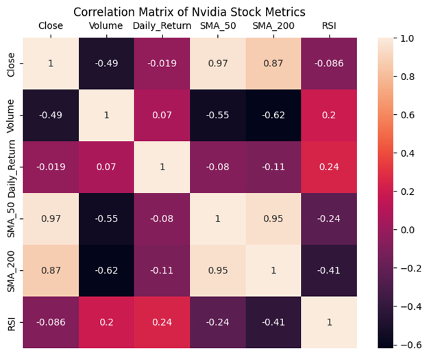
- Close Price & SMAs: A strong positive correlation suggests that Nvidia's stock exhibits trend-following behavior, aligning with the moving average patterns observed.
- Close Price & RSI: A negative correlation supports a mean-reversion tendency, where price pullbacks occur after overbought conditions.
- Volume & Daily Returns: Moderate correlation suggests that higher trading volumes influence short-term price fluctuations but are not the dominant factor in price movement.
Statistical Analysis
Daily returns
- Mean: 0.3 %
- Volatility: 3.23 %
Hypothesis testing
- t-statistique: 2.58
- p-value: 0.01
Given the statistically significant p-value, Nvidia's daily returns deviate from a normal distribution, suggesting possible market inefficiencies or external factors driving the stock's performance.
Risk and Performance Metrics
- Annualized returns: 93.94 %
- Annualized Volatility: 51.32 %
- Sharpe ratio: 1.8304 (indicating strong-adjusted returns)
Drawdown Analysis
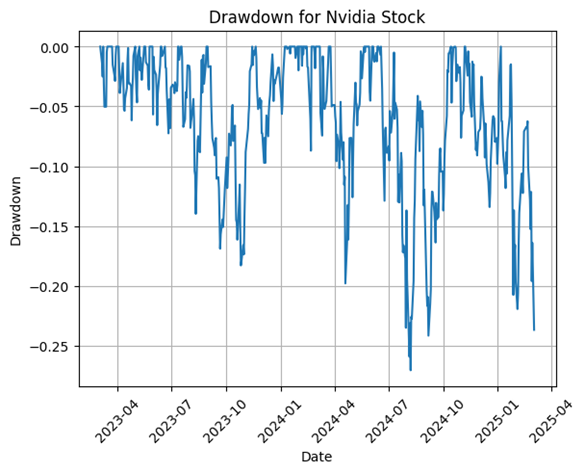
Nvidia experienced frequent and significant drawdowns, with a maximum drawdown of -27.05%. This highlights the stock's high volatility, meaning investors should prepare for sharp price swings. The period following the earnings announcement showed a significant price movement, contributing to the overall drawdown pattern.
Market Outperformance
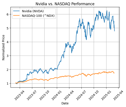
Over the past two years, Nvidia has outperformed the NASDAQ-100, reflecting investors confidence in its growth potential within AI and semiconductor markets.
Price Prediction Analysis
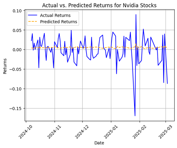
- Mean Squared Error: 0.001115 (indicating a relatively accurate model)
- Model Coefficient: -0.0565
- Intercept: 0.005
The model suggests a potential price correction, but further validation is necessary to confirm predictive power.
Monte Carlo Simulation for Future Price Estimates
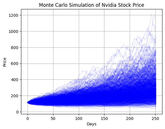
- Expected price after one year: $300.39
- Standard deviation (risk): $157.17
The wide standard deviation underscores significant uncertainty in Nvidia's future price movements, reinforcing the importance of risk management strategies for investors.
Next Steps for investors
- Monitor the SMA crossover to confirm a potential downtrend.
- Assess AI market developments and Nvidia's positioning.
- Diversify holdings to mitigate Nvidia-specific risks.
- Analyze the details of the recent earnings report and management's forward guidance to inform investment decisions.
Python Code for Data Analysis
                import yfinance as yf
                import pandas as pd
                import numpy as np
                import matplotlib.pyplot as plt
                import seaborn as sns
                from scipy import stats

                # NVDA stock data
                nvda_data = yf.Ticker("NVDA")
                nvda = nvda_data.history(start='2023-03-03', end='2025-03-04')

                # Benchmark data
                nasdaq_data = yf.Ticker("^NDX")
                nasdaq = nasdaq_data.history(start='2023-03-01', end='2025-03-01')

                # Technical Indicators
                nvda['SMA_50'] = nvda['Close'].rolling(window=50).mean()
                nvda['SMA_200'] = nvda['Close'].rolling(window=200).mean()
                nvda['EMA_12'] = nvda['Close'].ewm(span=12, adjust=False).mean()
                nvda['EMA_26'] = nvda['Close'].ewm(span=26, adjust=False).mean()
                nvda['MACD'] = nvda['EMA_12'] - nvda['EMA_26']
                nvda['Signal_Line'] = nvda['MACD'].ewm(span=9, adjust=False).mean()
                nvda['RSI'] = 100 - (100 / (1 + nvda['Close'].diff(1).clip(lower=0).rolling(14).mean() / nvda['Close'].diff(1).clip(upper=0).abs().rolling(14).mean()))

                # Daily returns and cumulative returns
                nvda['Daily_Return'] = nvda['Close'].pct_change()
                nvda['Cumulative_Return'] = (1 + nvda['Daily_Return']).cumprod() - 1

                # Visualisation of stock price and moving averages
                plt.plot(nvda.index, nvda['Close'], label='NVDA Close Price')
                plt.plot(nvda.index, nvda['SMA_50'], label='50-day SMA')
                plt.plot(nvda.index, nvda['SMA_200'] , label='200-day SMA')
                plt.title('Nvidia Stock Price with Moving Averages')
                plt.xlabel('Date')
                plt.xticks(rotation=45)
                plt.ylabel('Price (USD)')
                plt.grid(True)
                plt.legend()
                plt.show()

                # Visualisation of MACD
                plt.plot(nvda.index, nvda['MACD'], label='MACD')
                plt.plot(nvda.index, nvda['Signal_Line'], label='Signal Line')
                plt.title('MACD for Nvidia Stock')
                plt.xlabel('Date')
                plt.xticks(rotation=45)
                plt.ylabel('MACD')
                plt.grid(True)
                plt.legend()
                plt.show()

                # Visualisation of RSI
                plt.plot(nvda.index, nvda['RSI'], label='RSI')
                plt.axhline(y=70, color='r', linestyle='--')
                plt.axhline(y=30, color='g', linestyle='--')
                plt.title('RSI for Nvidia Stock')
                plt.xlabel('Date')
                plt.xticks(rotation=45)
                plt.ylabel('RSI')
                plt.grid(True)
                plt.legend()
                plt.show()

                # Correlation matrix
                correlation_matrix = nvda[['Close', 'Volume', 'Daily_Return', 'SMA_50', 'SMA_200', 'RSI']].corr()
                plt.figure(figsize=(8,6))
                sns.heatmap(correlation_matrix, annot=True)
                plt.gca().xaxis.set_ticks_position('top')
                plt.title('Correlation Matrix of Nvidia Stock Metrics')
                plt.show()

                # Basis Statistical analysis
                print("Summary Statistics of Daily Returns:")
                print(nvda['Daily_Return'].describe())

                # Hypothesis testing
                t_stat, p_value = stats.ttest_1samp(nvda['Daily_Return'].dropna(), 0)
                print(f"\nOne-sample t-test results:")
                print(f"t-statistic: {t_stat}")
                print(f"p-value: {p_value}")

                # Risk metrics
                annualized_return = nvda['Daily_Return'].mean() * 252
                annualized_volatility = nvda['Daily_Return'].std() * np.sqrt(252)
                sharpe_ratio = annualized_return / annualized_volatility

                print(f"\nRisk Metrics:")
                print(f"Annualized Return: {annualized_return:.4f}")
                print(f"Annualized Volatility: {annualized_volatility:.4f}")
                print(f"Sharpe Ratio: {sharpe_ratio:.4f}")

                # Drawdowns
                nvda['Peak'] = nvda['Close'].cummax()
                nvda['Drawdown'] = (nvda['Close'] - nvda['Peak']) / nvda['Peak']

                plt.plot(nvda.index, nvda['Drawdown'])
                plt.title('Drawdown for Nvidia Stock')
                plt.xlabel('Date')
                plt.xticks(rotation=45)
                plt.ylabel('Drawdown')
                plt.grid(True)
                plt.show()

                print(f"\nMaximum Drawdown: {nvda['Drawdown'].min():.4f}")

                # Visualisation of cumulative returns
                plt.plot(nvda.index, nvda['Cumulative_Return'])
                plt.title('Cumulative Returns for Nvidia Stock')
                plt.xlabel('Date')
                plt.xticks(rotation=45)
                plt.ylabel('Cumulative Return')
                plt.grid(True)
                plt.show()

                # Comparison to benchmarck
                # Normalized prices
                nvda['Normalized'] = nvda['Close'] / nvda['Close'].iloc[0]
                nasdaq['Normalized'] = nasdaq['Close'] / nasdaq['Close'].iloc[0]

                plt.plot(nvda.index, nvda['Normalized'], label="Nvidia (NVDA)")
                plt.plot(nasdaq.index, nasdaq['Normalized'], label="NASDAQ-100 (^NDX)")
                plt.title("Nvidia vs. NASDAQ Performance")
                plt.xlabel("Date")
                plt.xticks(rotation=45)
                plt.ylabel("Normalized Price")
                plt.grid(True)
                plt.legend()
                plt.show()

                # Price prediction (Machine Learning)
                from sklearn.linear_model import LinearRegression
                from sklearn.metrics import mean_squared_error

                #prepare data
                nvda['Return'] = nvda['Close'].pct_change()
                nvda['Lagged_Return'] = nvda['Return'].shift(1)

                ml_data = nvda.dropna(subset=['Return', 'Lagged_Return'])

                # Features X and target y
                X = ml_data['Lagged_Return'].values.reshape(-1, 1)
                y = ml_data['Return']

                # Train-test split
                train_size = int(len(X) * 0.8)
                X_train, X_test = X[:train_size], X[train_size:]
                y_train, y_test = y[:train_size], y[train_size:]

                # Train the linear regression model
                model = LinearRegression()
                model.fit(X_train, y_train)

                # Predictions and evaluation of the model
                y_pred = model.predict(X_test)
                mse = mean_squared_error(y_test, y_pred)

                print(f"Mean Squared Error (MSE): {mse:.6f}")
                print(f"Model Coefficient: {model.coef_[0]:.4f}")
                print(f"Model Intercept: {model.intercept_:.4f}")

                plt.plot(y_test.index, y_test, label="Actual Returns", color='blue')
                plt.plot(y_test.index, y_pred, label="Predicted Returns", color='orange', linestyle='--')
                plt.title("Actual vs. Predicted Returns for Nvidia Stocks")
                plt.xlabel("Date")
                plt.xticks(rotation=45)
                plt.ylabel("Returns")
                plt.grid(True)
                plt.legend()
                plt.show()

                # Monte Carlo Simulation for risk assesment
                # Parameters
                num_simulations = 1000
                num_days = 252
                last_price = nvda['Close'].iloc[-1]
                mean_return = nvda['Return'].mean()
                std_return = nvda['Return'].std()

                np.random.seed(42)      # for reproducibility

                simulated_prices = np.zeros((num_days, num_simulations))

                for sim in range(num_simulations):
                    prices = [last_price]
                    for day in range(1, num_days):
                        random_return = np.random.normal(mean_return, std_return)
                        prices.append(prices[-1] * (1 + random_return))
                    simulated_prices[:, sim] = prices[:num_days]

                for sim in range(num_simulations):
                    plt.plot(simulated_prices[:, sim], alpha=0.1, color='blue')
                plt.title("Monte Carlo Simulation of Nvidia Stock Price")
                plt.xlabel("Days")
                plt.ylabel("Price")
                plt.grid(True)
                plt.show()

                # Expected price and risk metrics
                expected_price = simulated_prices[-1].mean()
                price_std = simulated_prices[-1].std()
                print(f"Expected Price After 1 Year: ${expected_price:.2f}")
                print(f"Risk (Standard deviation of final prices): ${price_std:.2f}")